Parametric Functions in 3 dimensions
You can tell which axis is x and which is y by the right hand convention. If you push the positive x axis into the positive y axis by curling the fingers of your right hand, your thumb points in the direction of positive z.
Coordinate systems
First a digression to make sure that we all understand graphing in three dimensions. (For now, we will focus on rectangular coordinates.)
Whereas before we located points in a plane by determining distances from the origin along two perpindicular lines, we now do the same thing -- and more. First, imagine rotating the x-y plane so that it moves from being perpendicular to your gaze to being "flat" with your gaze. Then think of that plane being located in space.
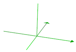
We locate a point in space by first locating a point in the x-y plane (as before) that is right "under" (or "over") the point in question, then we go some distance above or below the x-y plane to reach it. That distance is the point's z coordinate.
We represent a point in space with an ordered triple. In GC you get an ordered triple by typing cntrl/cmd-3. You can plot points and generate vectors in the usual way, as in:
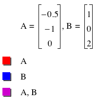
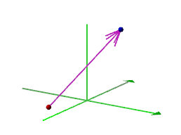
Point A has an x-coordinate of -0.5, a y-coordinate of -1, and a z coordinate of 0 (that is, it is in the x-y plane). Point B has an x-coordinate of 1, a y-coordinate of 0, and a z-coordinate of 2 (that is, it is in the x-z plane.
Space Curves
You can create curves in space (3-d) by using constants and parameters to define the coordinates of points on the curve. You define the points' coordinates parametrically, meaning that each coordinate is a function of the same variable. For example,
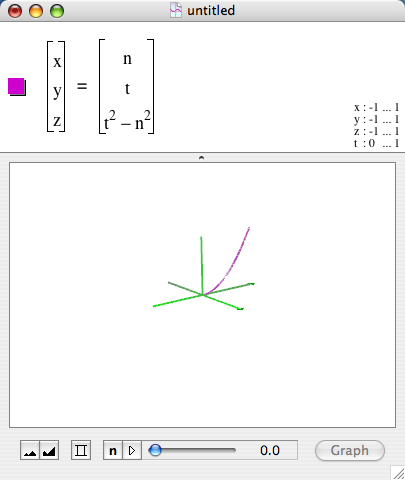
To interpret this graph you must keep in mind the scope of variation among n, t, and t2 - n2: first n takes a value, say 0. This fixes the to-be-graphed points' x-coordinates at 0. Then t varies in its domain (in the above diagram it varies from 0 to 1). As t varies, the x-coordinate remains 0 and the y-coordinates are the values of t. Finally, as t varies, the points' z-coordinates are the values of t2- n2. So, for n=0 and t varying from 0 to 1, the points generated are as in the table below. The table shows what the graph is made of -- points that have 0 as their x-coordinate, their y-coordinates range from 0 to 1, and their z-coordinates are t2 - n2.
| n |
t |
t^2 - n^2 |
| 0 |
0.1 |
0.01 |
| 0 |
0.2 |
0.04 |
| 0 |
0.3 |
0.09 |
| 0 |
0.4 |
0.16 |
| 0 |
0.5 |
0.25 |
| 0 |
0.6 |
0.36 |
| 0 |
0.7 |
0.49 |
| 0 |
0.8 |
0.64 |
| 0 |
0.9 |
0.81 |
| 0 |
1.0 |
1.00 |
Here is another table with n = 1.
| n |
t |
t^2 - n^2 |
| 1 |
0.1 |
-0.99 |
| 1 |
0.2 |
-0.96 |
| 1 |
0.3 |
-0.91 |
| 1 |
0.4 |
-0.84 |
| 1 |
0.5 |
-0.75 |
| 1 |
0.6 |
-0.64 |
| 1 |
0.7 |
-0.51 |
| 1 |
0.8 |
-0.36 |
| 1 |
0.9 |
-0.19 |
| 1 |
1.0 |
0.00 |
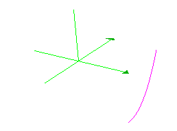
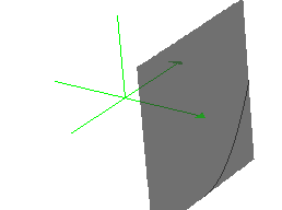
This table goes with a curve that is in a plane parallel to the y-z plane that passes through x=1, as shown below. The graph on the left is of  . The graph on the right is the same, but also shows the plane parallel to the y-z plane passing through x=1. Another way to think of this function is think of it as a curve defined over the segment in the
Curves in 3-d needn't be defined over lines or line segments. They can be defined over any path in the x-y plane (or x-z, or y-z). Play (double-click) the movie below to see how points are located. In this movie, each point on the unit circle with coordinates (x,y) is elevated to a height of z = 1 - xy.
The coordinates of the circle can be represented in a number of ways. Two of them are:
 and
and  , 0 < t <=1.
In the second case, points in the plane are given in polar coordinates. The coordinates of the space curve can be represented in both cases by letting the z-cordinate be 1 - (cos2πt)(sin2πt).


 . The graph on the right is the same, but also shows the plane parallel to the y-z plane passing through x=1. Another way to think of this function is think of it as a curve defined over the segment in the
 and
and  , 0 < t <=1.